Puredata for Analytics: Identify and resolve skew.

Answer

Database performance issues are sometimes caused by SKEW. Skew is used in this paper to refer to the occurrence of an unbalanced amount of work taking place on 1 or a subset of all active dataslices. Skew can mitigate the great performance advantage of the parallel architecture, which is a cornerstone of the PureData System for Analytics appliance. It may manifest itself in two forms… storage skew and processing skew. Each may cause a negative performance impact for the subject query and the entire system’s workload. This will address how to identify and options to resolve both storage and processing skew.

What is storage skew? When data is loaded to a table, the rows are distributed to a particular dataslice based on the defined distribution key, assuming distribution is not defined as random. The dataslices holding a larger count of table rows will generally work longer, harder, and consume more resources to complete its job. These dataslices can become a performance bottleneck for the queries. This uneven distribution of table rows is known as storage skew.

What is processing skew? A query will need to process table data in various ways to produce the final result set. Along the way, intermediate tables will be used as a way to filter, project, sort, and aggregate data, along with broadcasting and redistributing data. These intermediate tables may produce an uneven distribution, which can negatively impact the benefits of parallelism. Because this happens as a result of how the data is processed within the query, this is known as processing skew.


Indicators that skew might exist

1) Storage skew

Skew within data at rest (storage skew) is the most straightforward to identify. The goal is to find those tables that have a significant gap in disk space used between the largest dataslice and the smallest. We provide multiple methods for finding this.

Software Support Toolkit (/nz/support/bin):

nz_skew will list all tables on the system in which the largest dataslice has 100MB more disk used than the smallest. The 100MB value is the default, but is configurable. It will list the appropriate metrics along with the most highly skewed dataslice. See “nz_skew –h” for more information.

nz_record_skew will check skew for a particular table. As a best practice, only use this script to view the skewness of an individual table that you have suspicions about. Running this against all tables in a database can take an exorbitant amount of time. See “nz_record_skew –h” for more information.


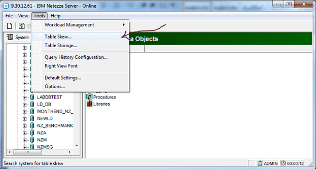
IBM Netezza Administrator:

IBM Netezza Administrator will generate the same results as nz_skew, while using a GUI interface.





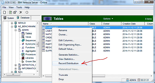
Within IBM Netezza Administrator, it is possible to drill down to the table level to get a more granular picture. This is similar content to nz_record_skew, but provides a graphical view using the GUI interface.




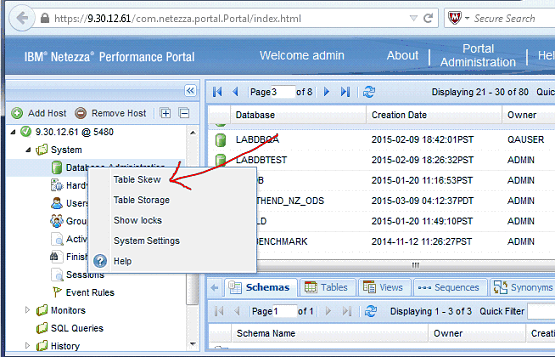
IBM Netezza Performance Portal:

IBM Netezza Performance Portal can produce the same storage skew reports as IBM Netezza Administrator. First, listing all skewed tables on the system….



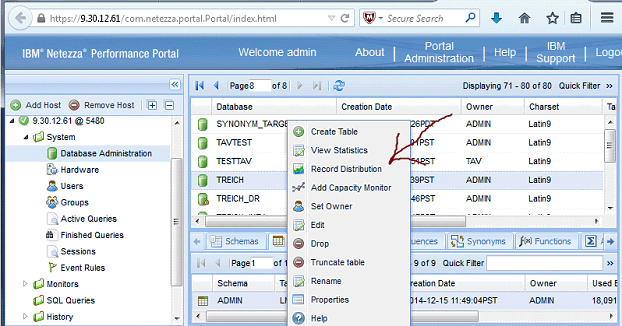
And, displaying the skewness at the table level…




2) Event Manager (Disk Full) notifications on 1 or a subset of dataslices

By default, the Event Manager is defined to send an alert when a particular dataslice has been allocated to 80% and again when it is allocated to 90%. The primary purpose of this event is to proactively warn that a dataslice is nearing full capacity, which would then prevent INSERT/UPDATE activity. But a byproduct of this is to identify storage skew. If a notification is sent for 1 or a small subset of dataslices, especially if the notification is for 90% full, whereas other dataslices have not produced an 80% notification, then it is likely that storage skew exists.



3) Resource utilization metrics

There are several places in which resource utilization metrics are exposed for analysis. This would include

· System View _V_SYSTEM_UTIL
· System View _V_SCHED_GRA_EXT
· System View _V_PLAN_RESOURCE and its permanent repository nz_query_history
· System View _V_PLAN_PROGRESS -or- Command: nzsqa progress
· Plan Files – snippet detail

In each of these repositories, there is some form of average disk I/O and maximum disk I/O. While these metrics are at the SPU level, as opposed to the dataslice level, this analysis can still be a valuable indicator if skew may exist. Keep in mind that the PureData Systems for Analytics architecture is such that all SPUs will not be managing the same number of dataslices*. On N100* models, there could be a 25% difference and on N200*/N300* models there could be a 20% difference. So, to identify real skew using these metrics, you would want to see something in the order of at least a 2-to-1 difference.

^* On a TwinFin, some SPUs will manage 6 dataslices while others will manage 8 dataslices. A Striper/Mako SPU will manage 32 or 40 dataslices. See the Notes section at the end of this document for further details.



4) nz_responders

The nz_responders utility, found in the Software Support Toolkit (/nz/support/bin), shows how a query snippet is responding against the community of dataslices as it is running. This utility is commonly used very early in any real-time performance analysis and could be your first signal that skew exists.

The nz_responders output of a balanced, non-skew affected snippet might look something like this…

Cur Time Plan #  Snippet   Time S/P  State  Busy Dataslices ...   SQL                          
======== ====== ========= ========= ======= ==== ================ ============================
15:33:05     83     (2/4)     34/35 RUNNING 240                   update product set part_numb

How can you tell this snippet is balanced? This happens to be a PDA appliance (N3001-010) with 240 dataslices. Under the Busy column, it shows a count of 240. This tells us that all dataslices are performing work.

However, if there is skew, the snippet might look something like this.

Cur Time Plan #  Snippet   Time S/P  State  Busy Dataslices ...   SQL                          
======== ====== ========= ========= ======= ==== ================ ============================
15:33:05     83     (2/4)     34/35 RUNNING 1    112              update product set part_numb

We see that not all 240 dataslices are busy… only one is… dataslice # 112. This one remaining dataslice is known as a laggard. It is still busy after the other dataslices have finished their work. A snippet cannot complete until all dataslices are finished, thus the query waits for this one dataslice before it can progress to the next snippet.

If nz_responders shows that the same dataslice(s) seems to be consistently lagging for extended periods of time, then you MAY be experiencing storage or processing skew.


What could cause nz_responders to indicate lagging dataslices for non-skew reasons?

nz_responders is often the most useful tool available to identify potential skew issues. But, this utility can report lagging dataslices that occur for reasons other than skew, such as Topology imbalance, Slow disk, and Disk failure/regen. It is important to understand how to diagnose these alternative causes of a lagging dataslice so that proper due diligence can be performed.

Topology imbalance
The PDA appliance is designed to support a balanced number of dataslices per hba port. If this becomes out of balance, then the dataslices assigned to an oversubscribed port may lag behind the rest of the dataslices. There are several ways to be made aware that a topology imbalance exists.

1. Event Manager’s Topology Imbalance event will generate a notification as an imbalance is recognized. Use the nzevent command or the IBM Netezza Administrator to confirm this event is enabled.
2. The System Health Check utility (nzhealthcheck) will report a topology imbalance. A good idea to run this utility at regular intervals.
3. The command “nzds show –topology” will report the current topology along with any imbalance issues

Generally, an “nzhw rebalance” or an nzstop/nzstart (in some cases in conjunction with a powercycle) will correct topology issues. If that does not balance the topology, then IBM Support should be engaged.

Disk failure/regen
PDA incorporates RAID 1 for user data. Disks work in pairs. The primary dataslice on DiskA is the mirror dataslice on DiskB and vice versa. When DiskA fails, then DiskB must service the load of 2 dataslices (double duty mode), causing both dataslices to lag. In addition, the spare disk that will take the place of DiskA is being built from the available dataslices on DiskB. This causes additional Disk I/O for DiskB, contributing to its already higher disk utilization rates. Thus, the dataslices involved with a disk failure and regeneration would lag the other dataslices. The command “nzds –issues” will show if the disk topology has a disk in double duty mode and/or is performing disk regeneration.

Slow disk
A disk that is experiencing performance degradation may consistently show up in nz_responders as lagging. A disk that is degraded will naturally complete its work slower than healthy disks. It is a best practice to periodically run the utility nzhealthcheck to proactively identify disks that may be physically degrading. On the flip side, if you see a disk that is consistently lagging in nz_responders, the cause of slow disk vs. skew cannot be confirmed in other ways, then run the utility nz_check_disk_scan_speeds (found in the Software Support Toolkit - /nz/support/bin) on the system while no other workload is accessing the dataslices. This can be run in various ways (see nz_check_disk_scan_speeds – h to display options) to isolate a slow disk.

To summarize, there are various disk/hardware related issues that may incorrectly appear to be skew related. For additional information regarding how to identify and resolve these types of performance issues check this “Netezza peformance diagnosis when hardware issue is suspected” technote.


How to differentiate storage skew from processing skew

When identifying skew using nz_skew or by way of an Event Manager alert, your problem is storage skew. When skew is suspected by nz_responders or in analyzing resource utilization metrics, the task becomes a bit more complicated. The first step would be to review the snippet of the query plan in which skew was identified.

Looking at the query plan file, does the “skewed” snippet begin with a ScanNode for a user table? See this example of a ScanNode that does reference a user table (TREICH.ADMIN.LMN):

1[00]: spu ScanNode table "TREICH.ADMIN.LMN" 270467 index=0 cost=17226 (j)
       -- Cost=0.0..22049.3 Rows=10.4K Width=4 Size=40.8KB Conf=90  [BT: MaxPages=17226 TotalPages=51670] (JIT-Stats) {(C1)}
       -- Cardinality LMN.C1 300 (JIT)
1[01]: spu RestrictNode (non-NULL)
       -- (C3 = 56321)

If so, then it could be storage skew. In addition, this example shows the JIT Stats estimate indicating that 1/3^rd of the total pages to be accessed will come from one dataslice (MaxPages / TotalPages). This can lend credence to the suspicion of this table being skewed. Table skewness can be confirmed by using one of the tools listed above to view table level storage skew. If the table shows a fairly equitable distribution of rows, then the problem is likely processing skew.

If the snippet exhibiting skew does not begin with a ScanNode of a user table, then you have processing skew.


How to address storage skew

If a table is found to have significant storage skew, it MAY need to be addressed. When a table is created, it is defined with a distribution key or defined to be distributed on random. If the table is distributed on random, the rows will be uniformly distributed across the dataslices. But, when the table is defined with a distribution key (1 to 4 columns) data has the opportunity to be unevenly distributed. Obviously, to resolve this, a new distribution key would need to be chosen. To build a table with minimal skew, the distribution key should have a high level of distinctness. This needs to be balanced with a competing goal for defining distribution keys – keep the column count small, ideally 1^*. Choose column(s) that have high cardinality. By including columns of low cardinality (T/F, 1/0, M/F, Codes) the degree of distinctness will not increase significantly enough to aid in producing an even row distribution.

To analyze columns that would be good candidates from a distinctiveness perspective, for the distribution key use the nz_table_analyze utility, found in the Software Support Toolkit (/nz/support/bin). This will show the uniqueness of each column, along with how lumpy the data is (one or a set of values abnormally common).

Another way to test the skew level of a new distribution key is to create a copy of the table using that new distribution key.

CREATE TABLE <new-table> AS SELECT * FROM <current-table> DISTRIBUTE ON (<new-dist-key>);

It is important to not sacrifice co-located join operations in order to eliminate storage skew. If two tables are distributed on the same columns and are also joined on those columns or a superset of those columns, a join of those two tables can be completed local to its SPU without network traffic or communication between SPUs. Distributing those two tables on the same columns may come at the expense of skew on one or both of those tables. But, being able to co-locate joins in this manner can often outweigh the expense of dealing with storage skew. In fact, the primary purpose of choosing a distribution key is to exploit the opportunities for co-located joins. Other purposes of having a distribution key could include improving efficiency of aggregations and allowing for single slice optimization. There is no need to pick a distribution key, just for the sake of having a distribution key. If, after careful analysis, there are no valid reasons discovered for a table to have a distribution key, then distributing on Random would be a good choice. As always, benchmark testing with a representative workload is a good barometer as to which approach to take.

^* Reasons for keeping the column count small in a distribution key is outside the scope of this document. At a high level, fewer columns included in a distribution key will optimize the opportunity for co-located joins.


How to address processing skew

Processing skew can be more difficult to address. And a solution may come at a cost (time to test and implement, impact on other queries referencing the same table, etc.). If the nature of an identified case of processing skew is neither consistent nor unacceptable, then consider leaving it be. But, if processing skew leads to unacceptable performance of a query or the processing skew creates a hot dataslice that impacts the concurrent workload in an unacceptable way, then a resolution needs to be found and implemented.

First, confirm with the developer of the query that the SQL is correct. For example, check that there are no unexpected, unnecessary, or missing joins. Also, check that the WHERE clause is constructed as expected. Have the developer make any necessary corrections.

The PDA Query Planner attempts to avoid processing skew. On occasion, because of out of date data statistics, the planner may make a choice that inadvertently introduces processing skew. That may be evident by looking at the plan file and finding where the query planner reported statistic estimates that were inaccurate. Trace that back to the tables involved, determine if any have out of date statistics. If so, run the GENERATE STATISTICS utility on the necessary tables.

If a Fact table is distributed on one dimension and queries are often based on that dimension, then processing skew could arise. Consider this example: A fact table called SALES is distributed on one column called STORE. There are 2000 unique stores and the SALES data seems to be fairly evenly distributed across the dataslices. But, reports based on a single store’s results are commonly requested. It is noticed that these reports tend to exhibit processing skew, as the majority of the work happens on the dataslice in which its store has been distributed to. To resolve this, a new distribution key should be chosen to allow rows for each distinct store to be spread across all dataslices.

In those cases in which a Fact table has an attribute that is managed in an unnatural way, processing skew could develop. One example of this could be on an ORDER table in which the TRANSACTION_CANCEL_DATE column is set to 9999-12-31 for those orders that have not been cancelled. Processing cancellations by date range could funnel all of these uncancelled orders to one dataslice as the query planner may not be aware of this unnatural data management. Another example could be on that same ORDER table having an attribute called CUSTOMER_ACCT. For all orders in the system that are not associated with a specific customer (internal orders), the value of 0 is stored. Joining this table to a Customer dimension table on CUSTOMER_ACCT could then lead to processing skew. Both of these examples could be resolved by a change to the database design or ETL process. For instance, if both of these columns are defined as NULLABLE and the value of NULL is used in these special cases rather than an out of range default value, then the query planner can intelligently avoid skew by excluding these rows appropriately.

The PDA Query Planner will choose how intermediate tables are distributed. It will factor in the cost of moving data with the cost of efficiently performing joins. It could be possible that an intermediate table will be built with significant skew, in which there are no viable ways found to mitigate that. In a case like this, the query could be split up so that the first step of the query builds the intermediate table as a temporary table in which you define the distribution key. This gives you greater control of how the data is physically distributed on disk. The second step of the query uses that temporary table to complete the query.



Notes:

It is extremely rare to achieve perfect balance and sometimes counterproductive to do so. Some amount of skew (storage or processing) is acceptable and expected.

All SPUs will not manage the same number of dataslices. The appliances are optimized for a TwinFin SPU to manage 8 dataslices and a Striper/Mako SPU to manage 40 dataslices. In each model, there will be SPUs that manage fewer dataslices than the optimized number, but that is as designed to provide capacity to absorb a SPU failure without impacting performance. So, the amount of work for each SPU can vary, causing a set of dataslices from some SPUs to finish slightly faster than the set of dataslices from other SPUs. The system view _V_DSLICE can shed light on the dataslice to SPU mapping.